How certain are we about the parameters that we estimate in our population model? Is that volume of distribution that NONMEM gave us really 10 liters with a clearance of 5 L/h? Or can it also be 9L and 6L/h respectively? And what will the impact of this uncertainty be on your simulations?
This is the issue that we call parameter uncertainty.
This post will provide a brief insight in what the effect of parameter uncertainty may be on your model simulation. However, it is definitely not a complete guide to all aspects of the different ways to do this and the pitfalls and limitations associated with it.
Objectives
- Perform a simulation in which we want to show the confidence interval around the mean and 5-95 percentiles concentration-time profile in the first 12h after dosing
- Modify the covariance matrix to show what the impact would be of having a 15%, 30%, or 50% RSE on all parameters
This blog post was inspired by the YouTube video of Kyle Baron on the probability of technical success simulation (https://www.youtube.com/watch?v=F_oM1V4Lp90), but it goes more back to basic.
Introduction
What we always try to achieve is to develop a model with very low relative standard errors on our parameters (RSE). These RSE’s indicate the confidence we have in our estimated parameters and is exactly what I describe in the first paragraph, how certain are we about the estimated parameters. High or low RSE’s on your parameters can be caused by the number of observations, sample size, the sampling schedule (no samples in the absorption phase will make it difficult to estimate your absorption rate constant), the number of parameters in the model, the wrong model, etc.
This is also a criteria when you judge published population PK/PD models. However, what is actually the impact of high or low RSE’s on our model predictions? And what do you think is an acceptable cut-off?
In order to study this and include parameter uncertainty in our simulation, we can use the covariance matrix that is generated by NONMEM.
“Covariance is a measure of how changes in one variable are associated with changes in a second variable. Specifically, covariance measures the degree to which two variables are linearly associated.”
https://stats.stackexchange.com/questions/29713/what-is-covariance-in-plain-language
This covariance matrix not only gives the variance of the parameters itself but also the covariance with the other parameters. We can use this matrix to perform the best/most realistic simulations based on our model.
If you want to simulate a published model and the covariance matrix is not given, you can create the matrix yourself by calculating the variance of each parameter and setting the off-diagonals to 0. This does however create some additional bias since it does not take into account the covariance. If the RSE is given in the parameter table (as is hopefully done…), the variance can be calculated by:
SE = RSE*Parameter_Estimate
Variance = SE**2
We can then create the same matrix which we could use in the functions below by:
cov.matrix<-diag(Variance1,Variance2,Variance3)
Example model
A simple 1-compartment model with 2 dosing groups was used for this simulation from which data was simulated and re-estimated. The exploratory PK profiles look as follows:

Estimation of our model resulted in the following parameter estimates, with the RSE between [ ]:
- KA 0.679/h [2.2%]
- V1 15.2L [4.29%]
- CL 6.74L/h [8.61%]
We can see that RSE's are very accurate and all below 10%. The RSE's on the 2 included ETA's on the volume of distribution and the clearance were 43% and 23%, indicating higher uncertainty in these parameters.
If we would use these parameter estimates, without the inclusion of any parameter uncertainty, it would simulate a distribution like this:

This would assume that 90% of the individuals would have a Cmax between 1.6 and 3.7 with the mean maximal concentration around 2.2.
The question that would arise from a simulation like this is: if we would perform a new study, in a large number of subjects, how certain are we that the mean Cmax will be above 2?
As an answer, we just can't say anything about that from the current simulation!
Simulating new parameter sets with uncertainty
First of all, let's load some libraries that we will need:
library(dplyr)
library(mrgsolve)
library(ggplot2)
We will use the mvrnorm function in R to do our simulation. This functions needs the number of simulations we want to perform (n), the mean values of the estimated parameters (mu) and the covariance matrix (Sigma).
We will obtain the mean values of the parameters, also called the parameter estimates, from the .ext file generated by NONMEM at the end of each run. We will select the row where the Iteration == -1E9, which shows the final results.
est <- read.csv(paste(mod,".ext",sep=""), header=TRUE, skip=1, sep="") %>%
  filter(ITERATION == -1E9)
Since we are only interested in the parameter columns, we can delete the ITERATION and OBJ column from this object.
est$ITERATION <- NULL
est$OBJ <- NULL
We can load the covariance matrix from the .cov file, also generated by NONMEM (if the covariance step was successful). It is adviced that you specify MATRIX=R in the $COV block, this calculates the standard errors based on the Fisher information matrix. Then, convert it to a data.matrix
## Read in covariance matrix generated by NONMEM
cov <- read.csv(paste(mod,".cov",sep=""), header=TRUE, skip=1, sep="")
# Remove NAME column
cov$NAME <- NULL
## Create a matrix
cov<-data.matrix(cov)
Now, we have all the information to use mvrnorm. We can call the function with all the objects we just defined.
#### Number of simulated parameter sets
nsim <- 1000

### mvrnorm simulation based on covariance matrix
sim_parameters <- mvrnorm(n = nsim, mu=as.numeric(est), Sigma=cov, empirical = TRUE)
colnames(sim_parameters) <- colnames(est)
Pirana software also has a function that generates this first part of the script for you! This function will hard code the parameter estimates in the R-script. However, the scripts presented here go back to the files generated by NONMEM and is therefore not dependent on Pirana.
During your simulation of new parameter sets, one problem that you might face is that some simulated parameters will be negative due to the normal distribution. In this case, we will need to remove them from the parameter sets. This will however reduce the number of parameter sets that we will simulate. If the RSE is much higher than 50%, quite a high proportion of your simulated parameters may be negative and you should think about how to account for this. This could be done by specifying your parameters as KA = EXP(THETA(1)), allowing THETA(1) to go below 0. In that scenario, it doesn't matter that the simulated parameters are below zero! Just make sure that this EXP(THETA(1)) is also simulated in your model code.
## No negative values are allowed --> Remove them from all tables
sim_parameters<- as.data.frame(sim_parameters)
has.neg <- apply(sim_parameters, 1, function(row) any(row < 0)) ## Check for negative values
if(length(has.neg[has.neg == TRUE])>0){
  sim_parameters <- sim_parameters[-which(has.neg),] # Remove negative rows from df
}

### Update the nsim with the parameter sets higher than 0
nsim <- min(nrow(sim_parameters))
PK simulations with mrgsolve and parameter uncertainty
In order to start the simulations with different parameter sets, we need to define the number of simulations. In this scenario I choose an nsim of 1000 and 5000 individuals per simulations. As a rule of thumb, if you look at the generated graphs and see a smooth curve, you probably have simulated enough.
For mrgsolve, we first need to load in our model, the .cpp file of a basic 1-compartment model you can find below:
$PARAM
TVKA=1, TVVC=1, TVCL = 1

$CMT GUT CENT

$MAIN
double KA = TVKA;
double VC = TVVC*exp(ETA(1));
double CL = TVCL*exp(ETA(2));

double k10 = CL/VC;

$OMEGA 0 0

$SIGMA @labels PROP
0

$ODE
dxdt_GUT = -KA*GUT;
dxdt_CENT = KA*GUT - k10*CENT;

$TABLE
double IPRED = CENT/VC;
double DV = IPRED*(1+PROP);

while(DV < 0) {
  simeps();
  DV = IPRED*(1+PROP);
}

$CAPTURE IPRED DV
As you can see, our .cpp file has 3 parameters defined, the TVKA, TVVC, and TVCL.
In R, we need to load this model file and define an administration dataset (oral administration of a fixed dose).
We also initialize the grouped_summary object, which we will fill with the results from each replicate.
### Load in model for mrgsolve
mod <- mread_cache("popPK")

grouped_summary <- NULL

## Set dose
  dose <- 80

  # Create dosing rows
  Administration <-  as.data.frame(ev(ID=1:n_subjects,ii=24, cmt=1, addl=9999, amt=dose, rate = 0,time=0))
Then, iterating over all parameter sets, we attach the simulated THETA's to this dataframe which will be used in the model.
## Start the loop here. Do this for each parameter set
for(i in 1:nsim){

data <-Administration

## Set parameters in dataset
data$TVKA <- as.numeric(sim_parameters[i,1])
data$TVVC <- as.numeric(sim_parameters[i,2])
data$TVCL <- as.numeric(sim_parameters[i,3])
mrgsolve also requires a matrix of the omega's and sigma's, which we can easily create using the mrgsolve function as_bmat
## Generate omega matrix
omega.matrix <-   as_bmat(sim_parameters[i,],"OMEGA")[[1]]

## Generate sigma matrix
sigma.matrix <-   as_bmat(sim_parameters[i,],"SIGMA")[[1]]
Then, we can start the simulation with mrgsolve. We will simulate from time 0h - 12h with a delta of 0.1h.
  ###### Perform simulation in mrgsolve
  out <- mod %>%
    data_set(data) %>%
    omat(omega.matrix) %>%
    smat(sigma.matrix) %>%
    mrgsim(start=0,end=12,delta=0.1, obsonly=TRUE)


  ### Output of simulation to dataframe
  df <- as.data.frame(out)
Calculating summary statistics and plotting
The result of our simulation are 1000 PK profiles from 0-12 hours. For each iteration of a parameter set, we want to know the mean, median, low 5% percentile and high 95% percentile. This will give us the 90% distribution of the data. We also add the replicate number to the results.
  ###### Calculate summary statistics
  sum_stat <- df %>%
    group_by(time) %>%
    summarise(Mean_C=mean(DV,na.rm=T),
              Median_C=median(DV,na.rm=T),
              Low_percentile=quantile(DV,probs=0.05),
              High_percentile=quantile(DV,probs=0.95)
    )  %>% mutate(rep = i)
We then bind the results of this replicate to the grouped_summary object.
  ########### Add the results per replicate to the summary object
  grouped_summary <- rbind(grouped_summary,sum_stat)
When we have iterated over all the parameter sets, we can start the calculation of the key numbers, the confidence interval in the mean and in the 5-95% percentile interval of the data.
This will show us, based on our NONMEM model, how certain we are of these numbers.
To calculate this, we group the data by time and summarise all the relevant parameters.
###### Calculate summary statistics over all replicates
sum_stat <- grouped_summary %>%
  group_by(time) %>%
  summarise(
    ## Mean distribution
            mean_low_percentile=quantile(Mean_C,probs=0.05),
            mean_high_percentile=quantile(Mean_C,probs=0.95),
            mean_SD_SE=sd(Mean_C,na.rm=T),
    ## Median distribution
            median_low_percentile=quantile(Median_C,probs=0.05),
            median_high_percentile=quantile(Median_C,probs=0.95),
    ## Low percentile distribution
            low_low_percentile=quantile(Low_percentile,probs=0.05),
            low_high_percentile=quantile(Low_percentile,probs=0.95),
    ## High percentile distribution
            high_low_percentile=quantile(High_percentile,probs=0.05),
            high_high_percentile=quantile(High_percentile,probs=0.95)
  )
This gives us the 90% confidence interval in these values. In this code, the mean_SD_SE has also been calculated if you rather want to plot this.
In order to plot these results, we take a similar approach to the confidence interval VPC. Generating a separate ribbon for each outcome of interest, the mean, 5% percentile and 95% percentile. The width of the ribbon will indicate how much confidence we have in these values based on our developed model.
ggplot(sum_stat, aes(time, mean_low_percentile)) +
  ## Grey distribution between extremes
  geom_ribbon(aes(ymin=low_low_percentile,ymax=high_high_percentile),fill='grey',alpha=0.8)+

  ## Low percentile distribution
  geom_ribbon(aes(ymin=low_low_percentile,ymax=low_high_percentile),fill='darkblue',alpha=0.85)+
  ## High percentile distribution
  geom_ribbon(aes(ymin=high_low_percentile,ymax=high_high_percentile),fill='darkblue',alpha=0.85)+

  ## Mean distribution
  geom_ribbon(aes(ymin=mean_low_percentile,ymax=mean_high_percentile),fill='darkred',alpha=0.75)+


  scale_x_continuous(name='Time (h)',expand=c(0,0))+
  scale_y_continuous(name='Concentration',limits=c(0,4.5))+
  ggtitle('90% confidence intervals around the mean and the 90% percentile intervals of the population','Dose = 80 mg')+
  theme(legend.position = "none")+
  theme_bw()
When we look at the results, we can see that there is a narrow band around the outcomes, indicating that we are quite sure about these values. What we can see is that if we would have a very high sample size in a new study, the mean Cmax would range between 2.0 and 2.4. This would give us a high level of confidence in the use of this model and the resulting simulations.
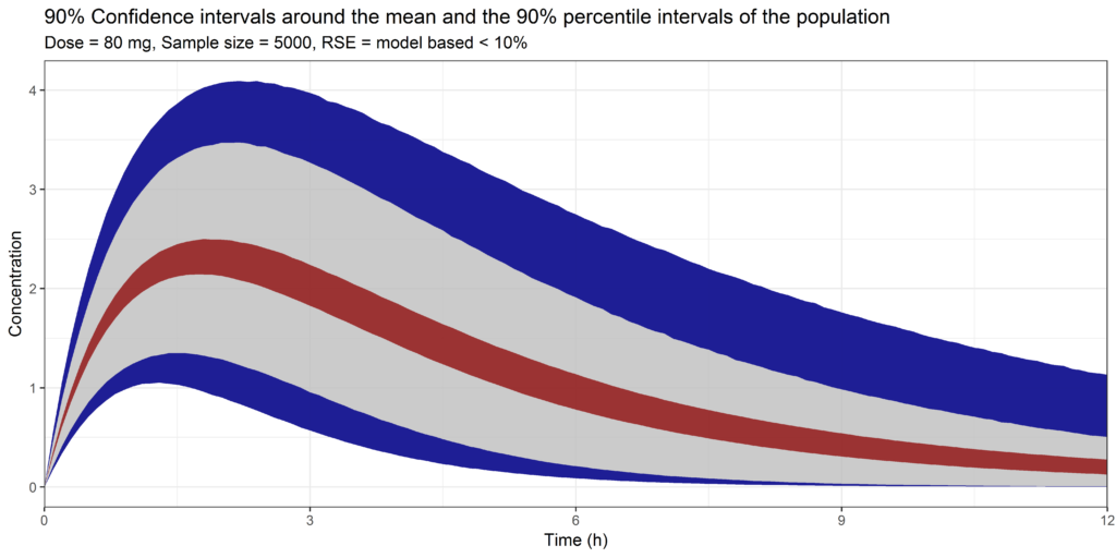
Simulation with parameter uncertainty, showing the 90% confidence interval around the mean and the 5% and 95% percentiles of the data. Simulated with the model based RSE's on all population parameters
Increasing our RSE to 15%, 30% or 50%
Having a narrow band around the previous simulation should not be that suprising. We had RSE's of < 10% on our population parameters to start with. However, we commonly see higher RSE's reported in literature so we can wonder how this would impact the simulations. In other words, if a simulation is being performed with a model with high RSE's, how much confidence do we have that the simulated profile will actually be what we will observe?
In order to do this, I used the same covariance matrix as in the previous example but now changed the first three diagonals to correspond with a 15%, 30% or 50% RSE of each population parameter. Keep in mind, this correspond to a simple 1-CMT model with the first three diagonals being the absorption rate constant, volume of distribution and clearance. A RSE of 15% or 30% would not be that unreasonable. A RSE of 50% would be quite high.
####### Change diagonals to 30% RSE on all parameters
cov[1,1] <- as.numeric((est[1]*0.3)**2)
cov[2,2] <- as.numeric((est[2]*0.3)**2)
cov[3,3] <- as.numeric((est[3]*0.3)**2)
When we perform exactly the same simulation, 1000 different parameter sets with 5000 subjects per simulation, the result for the 15% RSE is as follows:

Simulation with parameter uncertainty, showing the 90% confidence interval around the mean and the 5% and 95% percentiles of the data. Simulated with 15% RSE on all population parameters
And the results for the 30% RSE:
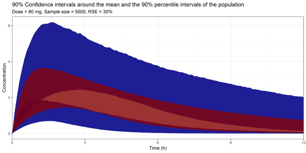
Simulation with parameter uncertainty, showing the 90% confidence interval around the mean and the 5% and 95% percentiles of the data. Simulated with 30% RSE on all population parameters
And the results for the 50% RSE:

Simulation with parameter uncertainty, showing the 90% confidence interval around the mean and the 5% and 95% percentiles of the data. Simulated with 50% RSE on all population parameters
We can clearly see a difference! Instead of those narrow bands we observed previously we actually can see an overlap between the mean and 5%-95% percentiles! Suddenly the 90% confidence interval around the Cmax ranges from 1 to 3.5!
This important information can't be retrieved from the simulation which did not include any parameter uncertainty. However, this is the figure that we commonly see reported in publications if simulations are performed with non-linear mixed effects models...
Clinical trial simulations
The simulations presented here are at the basis of performing a clinical trial simulation. With clinical trial simulations, we can use our population PK/PD model to identify the best sample size and dose that would, for example, give us a 90% probability of making the correct decision in our study. The only change in the script that we need to make is lower the sample size and run the simulation again. Having done the simulation with parameter uncertainty and a high sample sizes gives you a starting point to define new clinical trial strategies.
Conclusion
Pay attention to the estimated parameter uncertainty and the effects it may have on your model simulations! Also in literature models.
This post provides all the code necessary to load in your covariance matrix from NONMEM, create new parameter sets, simulate with mrgsolve and analyse your results. Performing these simulations will give much more information on how confident we are in our model simulations.
COMMENT
Any suggestions or typo’s? Leave a comment or contact me at info@pmxsolutions.com!
Download files
The NONMEM control stream, the covariance matrix, and the .ext file can be downloaded here. Make sure to remove the .txt extension (which is required to be downloaded) before you use the script for the analysis.


Can you post the ext file to reproduce the graph for learning purpose?
Thanks
Hello,
I have now added the NM model, the .ext and .cov file to reproduce the results of this post.
Good luck!
Thank you, this was very interesting. I was curious, when you set the dose (in this case 80mg fixed oral dose), how would setting the dose change, if you wanted to bring in weight, to calculate a weight-based dosing? Would there need to be a distribution set of patient-specific weights?
If you want to implement weight based changes in the dose, you can simulate and add a normal or uniform distribution of the covariate to the dataset on which you base the dose.
Example for a fixed dose as in the posted:
Administration <- as.data.frame(ev(ID=1:n_subjects,ii=24, cmt=1, addl=9999, amt=80, rate = 0,time=0))Add a weight for each subject:
Administration$WGT <- rnorm(n_subjects,70,8) # Mean of 70 with sd of 8Calculate new dose:
Administration$amt <- Administration$amt*Administration$WGTThank you for sharing! Question: psn has an option called “sir” to evaluate parameter uncertainty are these two approaches comparable/similar ?
Hello,
If I recall correctly, SIR is a method to estimate the level of parameter uncertainty. It provides an alternative to the non-parametric bootstrap approach (also available in PsN).
In this post, we use the estimated uncertainty in each parameter for subsequent simulations.
Hi, thank you for this very nice tutorial. Could you please comment on:
1) would truncation of the parameter (filtering out negative parameter values) affect the correlation/normal distribution assumption of parameters? I hope you can share the industry opinion and a plan B if this is a big concern.
2) for sequential PK PD models, if N = 500 for each of PK and PD simulations, then we would have 500*500 subjects in the PD simulation, which may become quite resource demanding. How would you handle that?
Thank you for your guidance!
Hi,
Two very interesting questions! I am not aware of any industry opinion regarding the trunctation of the parameter set. I would suggest checking the parameter set and determining the percentage of negative values and determine if the simulation would be biased after removal of these parameters. I would also say it is dependent on the parameter, of course, clearance and EC50 for example can’t be negative, but Emax can. So it really depends and the simulated parameter set but I would generally not be too bothered by it.
For question two, I would personally try to estimate the final model simultaneous to get the covariance matrix of all parameters. This would then include the interaction between PK and PD parameters. If this is not possible, 500×500 would be the next best thing. Using a mrgsolve simulation, with or without parallelization, would probably be done within 1 (long) coffee break.
This is a very informative tutorial on simulating PKPD models with parameter uncertainty. Very nice job!
I do not know whether the authors intend to write another blog on clinical trial simulations, as the authors mentioned using population PK/PD model simulations to identify the best sample size and dose in the current one.
I would like to represent all the PMX learners to appreciate the knowledge you shared, if you plan to write the blog.
Many thanks in advance!