It is difficult to grasp what non-linear mixed effects modelling software is actually doing when you start a run. Furthermore, the iteration prints that you see in the console (when using NONMEM) during a model run are also not very informative… Therefore, I wanted to visualize the model fit and the parameter distributions over time. This can be used in an educational setting where you for example need to explain modelling, a typical individual, inter-individual variability, residual error or variance.
This post will give all the code necessary to create the following GIF, with ODE simulations in R using the mrgsolve package and the output of a NONMEM run as input:
Load in the generated .ext file in R
There is a fairly easy way to get information on each iteration in NONMEM. First, we need to make sure that all the iterations are being printed by NONMEM by setting the PRINT statement in the $EST block to 1.
Then, the results of all iterations are being stored in the .ext file in your model directory. This consists of all the information we need, the THETA’s, SIGMA’s and OMEGA’s and we even get the objective function per iteration. However, this format can be quite troublesome to load in R.
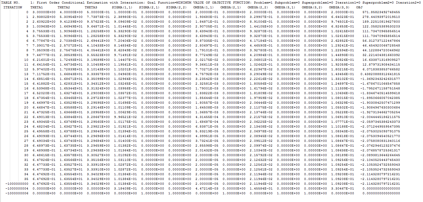
We cannot seperate it on comma’s (since there aren’t any), tabs, or spaces. Therefore, we need to use the fixed widths method, as is commonly applied in Excel. What you can see in the .ext file is that every column consists of 13 characters. Therefore, we can can determine the number of columns by reading in the file and divide it by 13. We need to do this since every model can have a different number of parameters.
extfile <- 'J:\\runEst.ext'

df_ext = readLines(extfile)
numbercolumn <- ceiling(nchar(df_ext[2])/13) # Round off to the top value
Then, we know how many columns we have, which we pass as the width argument in the read.fwf() function. We also want to add the headers which we add using the read.table() function.
df_ext_fwf <- read.fwf(extfile, widths = rep(13,each=numbercolumn), skip=2,
col.names = read.table(extfile, skip=1,nrow = 1, as.is = TRUE)[1, ])
If you look at the .ext file, there are some rows added on the bottom which can be useful for other purposes but which we do not use know, and should therefore be removed. We also want to clean the dataset so that we just have a few vectors that we need for our animation. These vectors consist of the parameter values per iteration.
 ### Remove negative iterations
df_ext_fwf <- df_ext_fwf [df_ext_fwf $ITERATION > 0,]

## Create vectors for the values we will use later
vector_ka <- df_ext_fwf [,2]
vector_Vd <- df_ext_fwf [,3]
vector_CL <- df_ext_fwf [,4]

vector_eta_ka<- df_ext_fwf [,8]
vector_eta_vd<- df_ext_fwf [,10]
vector_eta_cl<- df_ext_fwf [,13]

vector_sd_ka<- sqrt(df_ext_fwf [,8])
vector_sd_vd<- sqrt(df_ext_fwf [,10])
vector_sd_cl<- sqrt(df_ext_fwf [,13])

vector_eta_sigma<- df_ext_fwf [,5]

vector_OFV <- round(df_ext_fwf [,14],digits=3)
Simulate a user specified model with new THETA's and OMEGA's in mrgsolve
There are different methods to simulate ordinary differential equations (ODE) in R. However, recently I found out that mrgsolve is quite versatile and easy to work with. The notations of models are also very similar to NONMEM which made the transition for me very smooth. I also use it now in my Shiny apps for example. More information on the use of mrgsolve can of course be found on their website or on my different post.
But first, we need to define the model. We just use a very simple 1 compartment PK model in which we capture (report) the estimated concentrations by the model with residual error, and without. Then, we compile the model and save it in the object mod.
code <- '
$PARAM
TVCL = 1, TVVC=1, TVKA=1

$SET delta=0.1

$CMT GUT CENT

$MAIN
double KA = TVKA*exp(ETA(1));
double CL = TVCL*exp(ETA(2));
double VC = TVVC*exp(ETA(3));

double k10 = CL/VC;

$OMEGA 0 0 0
$SIGMA 0

$ODE
dxdt_GUT = -KA*GUT;
dxdt_CENT = KA*GUT – k10*CENT;

$TABLE
double CP = (CENT/VC)*(1+EPS(1));
double CP2 = (CENT/VC);

$CAPTURE CP CP2
'

## Compile and load the model
mod <- mcode_cache('ODEdef', code)
If we first look at the simulation of 1 iteration, we need to create a dataframe with the individual values of the clearance, volume and ka at this iteration. We specify a matrix for the omega's with no correlations present.
## Simulate 1000 subjects
idata <- data.frame(ID=1:1000)

## Specify the omegas and sigmas
omega <- cmat(vector_eta_ka[1],0, vector_eta_cl[1],0,0,vector_eta_vd[1])

sigma <- matrix(vector_eta_sigma[i])
Then, we set the dose of 100 mg for these individuals and add the population parameters (TVKA, TVCL, and TVKA) to the dataset. Again, the values of the current iteration (iteration i in this example) are used.
### Set dosing and interval

ev1 <- as.data.frame(ev(ID=1:1000,amt=100))

data <- merge(idata,ev1,by='ID')

data$TVKA <- vector_ka[i]
data$TVCL <- vector_CL[i]
data$TVVC <- vector_Vd[i]
We can then start the simulation by mrgsolve and transform the data to a new data frame (df) from which we can calculate the summary statistics. The simulation will run from 0 to 20h.
### Simulate data with mrgsolve

out <-
mod %>%
data_set(data) %>%
idata_set(idata) %>%
omat(omega) %>%
smat(sigma) %>%
mrgsim(end=20, obsonly=TRUE)

### Output data transformation
df <- as.data.frame(out)
We can include all these components in a loop that is performed for each iteration. We combine the data from all seperate iterations in the object df_all:
df_all <- NULL

for(i in 1:length(vector_ka)){

###############################################################
############### Dataset

## Simulate 1000 subjects with the iterated values
idata <- data.frame(ID=1:1000)

## Specify the omegas and sigmas
omega <- cmat(vector_eta_ka[i],0, vector_eta_cl[i],0,0,vector_eta_vd[i])

sigma <- matrix(vector_eta_sigma[i])

### Set dosing and interval

ev1 <- as.data.frame(ev(ID=1:1000,amt=100))

data <- merge(idata,ev1,by='ID')

data$TVKA <- vector_ka[i]
data$TVCL <- vector_CL[i]
data$TVVC <- vector_Vd[i]

### Simulate data with mrgsolve

out <- mod %>%
data_set(data) %>%
idata_set(idata) %>%
omat(omega) %>%
smat(sigma) %>%
mrgsim(end=20, obsonly=TRUE)

### Output data transformation
df <- as.data.frame(out)

df$Iteration <- i

df_all <- rbind(df_all,df)
}
Calculate summary statistics with the MRGSOLVE output
We use the dplyr piping function to quickly turn our dataframe that we got from mrgsolve in some summary statistics. We specify the groups (in this case per Iteration and per time), and calculate the median concentration, the 10-90% percentiles of the concentration with residual error (CP) included and without (CP2). This will be the dataframe that we use to create the animation in R.
sum_stat <- df_all %>%

group_by(Iteration,time) %>%

summarise(Conc=median(CP),
low25_RES=quantile(CP,probs=0.10),
high75_RES=quantile(CP,probs=0.90),
low25_IIV=quantile(CP2,probs=0.10),
high75_IIV=quantile(CP2,probs=0.90))
Create a GIF animation in R
To create the GIF in the way that I describe here, you need to have ImageMagick installed. If you can't install this software, there are many other ways to create GIF animations in R (e.g. https://ryanpeek.github.io/2016-10-19-animated-gif_maps_in_R/).
In order to create a GIF, we need to create 2 functions:
- draw.curve
- trace.animate
In short, these functions create the image that we want 35 times (for all the iterations) and paste them after each other so that an animation is created.
In the draw.curve function, we select the data that we need (so from a single iteration), and create a ggplot with the median line, a ribbon for the residual error distribution and a ribbon for the distribution with inter-individual variability. Then, we print this plot and the next iteration is started (that is done by trace.animate).
# GIF function which loops through all the iterations
draw.curve<-function(min){

## Select the iteration number
IT <- unique(sum_stat$Iteration)[min]

#############################################
# Concentration time profiles with 2 ribbons

p1<- ggplot(sum_stat[sum_stat$Iteration == IT,], aes(x=time,y=Conc)) +

## Add median line
geom_line(size=2,lty=’longdash’,color=’black’) +

## Add ribbon for variability including the residual error
geom_ribbon(aes(ymin=low25_RES, ymax=high75_RES, x=time, fill = '1'), alpha = 0.5)+

## Add ribbon for the ETA only
geom_ribbon(aes(ymin=low25_IIV, ymax=high75_IIV, x=time, fill = '2'), alpha = 0.6)+

# Set axis and theme
ylab('Concentration (mg/L)')+
xlab('Time after dose')+
theme_bw()+

# Add observations
geom_point(data=observations,aes(x=TIME,y=DV,group=ID))+

# Remove legend
theme(legend.position='none')+

# Use some grey colors
scale_fill_grey()+

## Add ggtitle with OFV
ggtitle('Typical individual',paste('Objective function value =', vector_OFV[min]))

print(p1)

}

# Function to iterate over the full span of iterations
trace.animate <- function() {
lapply(seq(1:length(unique(df_all$Iteration))), function(i) {
draw.curve(i)
})
}
We can execute the functions by calling the saveGIF() function (from the library(animation)) with some user specified arguments. Sometimes you also need to point R in the right direction to find the ImageMagick convert application which I did with ani.options. I have specified here that the interval between iterations is 0.6 seconds and the GIF should only play once (loop=1). You can also use the loop=0 argument to keep it playing forever.
#Save all iterations into one GIF ani.options(convert=’C:/Progra~1/ImageMagick-7.0.8-Q16/convert.exe’) saveGIF(trace.animate(), interval = .6, loop=1, movie.name='NONMEM_Model_fit_Pop_1x.gif',ani.width=750, ani.height=250)
However, we don't only want to visualize the PK profile in our animation. We also want to show the current iteration, a simulated parameter distribution, and the variance distributions. Then, we combine all ggplots on one page using the plot_grid function from cowplot. This is being achieved by the following piece of code:
draw.curve<-function(min){

## Select the iteration number
IT <- unique(sum_stat$Iteration)[min]

#############################################
# Concentration time profiles with 2 ribbons

p1<- ggplot(sum_stat[sum_stat$Iteration == IT,], aes(x=time,y=Conc)) +

## Add median line
geom_line(size=2,lty=’longdash’,color=’black’) +

## Add ribbon for variability including the residual error
geom_ribbon(aes(ymin=low25_RES, ymax=high75_RES, x=time, fill = '1'), alpha = 0.5)+

## Add ribbon for the ETA only
geom_ribbon(aes(ymin=low25_IIV, ymax=high75_IIV, x=time, fill = '2'), alpha = 0.6)+

# Set axis and theme
ylab('Concentration (mg/L)')+
xlab('Time after dose')+
theme_bw()+

# Add observations
geom_point(data=observations,aes(x=TIME,y=DV,group=ID))+

# Remove legend
theme(legend.position='none')+

# Use some grey colors
scale_fill_grey()+

## Add ggtitle
ggtitle('Typical individual',paste('Objective function value =', vector_OFV[min]))

###################################################
########### variance distributions around 0 – normal distribution

p2a <- ggplot(data = data.frame(x = c(-3, 3)), aes(x)) +
theme_bw() +
scale_x_continuous(limits=c(-3,3)) +
xlab('Variance distribution ka')+
stat_function(fun = dnorm, n = 101, args = list(mean = 0, sd = vector_sd_ka[min]),color=’darkred’,size=1) + ylab('')

p3a <- ggplot(data = data.frame(x = c(-3, 3)), aes(x)) +
theme_bw() +
scale_x_continuous(limits=c(-3,3)) +
xlab('Variance distribution Vd')+
stat_function(fun = dnorm, n = 101, args = list(mean = 0, sd = vector_sd_vd[min]),color=’darkred’,size=1) + ylab('')

p4a <- ggplot(data = data.frame(x = c(-3, 3)), aes(x)) +
theme_bw() +
scale_x_continuous(limits=c(-3,3)) +
xlab('Variance distribution CL')+
stat_function(fun = dnorm, n = 101, args = list(mean = 0, sd = vector_sd_cl[min]),color=’darkred’,size=1) + ylab('')

########### Parameter estimates distributions
#############################
normal_dis_ka <- rnorm(500, mean = 0, sd = vector_sd_ka[min])
ka_distr <- vector_ka[min]*exp(normal_dis_ka)
dis_ka <- as.data.frame(ka_distr)

p2 <- ggplot(data = dis_ka, aes(x=ka_distr)) +
theme_bw() +
geom_histogram(aes(y=..density..),color='black', fill='white')+
geom_density(alpha=.15, fill='#001158') +

scale_x_continuous(limits=c(0,10))+
xlab('Absorption rate constant (/h)')
#############################

#############################
normal_dis_vd <- rnorm(500, mean = 0, sd = vector_sd_vd[min])
vd_distr <- vector_Vd[min]*exp(normal_dis_vd)
dis_vd <- as.data.frame(vd_distr)

p3 <- ggplot(data = dis_vd, aes(x=vd_distr)) +
theme_bw() +
geom_histogram(aes(y=..density..),color='black', fill='white')+
geom_density(alpha=.15, fill='#001158') +

scale_x_continuous(limits=c(0,100))+
xlab('Distribution volume (L)')
#############################

#############################
normal_dis_cl <- rnorm(500, mean = 0, sd = vector_sd_cl[min])
cl_distr <- vector_CL[min]*exp(normal_dis_cl)
dis_cl <- as.data.frame(cl_distr)

p4 <- ggplot(data = dis_cl, aes(x=cl_distr)) +
theme_bw() +
geom_histogram(aes(y=..density..),color='black', fill='white') +
geom_density(alpha=.15, fill='#001158') +

scale_x_continuous(limits=c(0,20))+
xlab('Clearance (L/h)')
#############################

title <- ggdraw() +
draw_label(paste('Iteration:', IT),
fontface = ‘bold’,size=25)

plots_param <- plot_grid(p2,p3,p4,ncol=3)
plots_variance <- plot_grid(p2a,p3a,p4a,ncol=3)

plot_output <- plot_grid(title, p1,plots_param,plots_variance, ncol = 1, rel_heights = c(0.1, 1,1,1)) # rel_heights values control title margins

print(plot_output)

}
This animation can also be created only showing the typical individual, the typical + IIV, or the typical with IIV + residual as one distribution. These animations can be downloaded here:
NONMEM model fit animation - typical individual
NONMEM model fit animation - typical individual + IIV
NONMEM model fit animation - typical individual + RES
COMMENT
Any suggestions or typo’s? Leave a comment or contact me at info@pmxsolutions.com!