Introduction
Back in 2011, a very nice paper introducing the prediction corrected VPC was published by Bergstrand et al, titled:
“Prediction-Corrected Visual Predictive Checks for Diagnosing Nonlinear Mixed-Effects Models”
In the figure below you can see a comparison between a confidence interval VPC (ciVPC) on the left and a prediction corrected VPC (pcVPC) on the right. Due to the dose adaptions that were applied in this study, the ciVPC seems to show a model misspecification. However, when correcting for the individual predictions (which include these dose adaptions), the model actually seems to fit the data adequately. The paper really gives a nice overview in when to use this method for your model evaluation and is a recommended read for every modeller.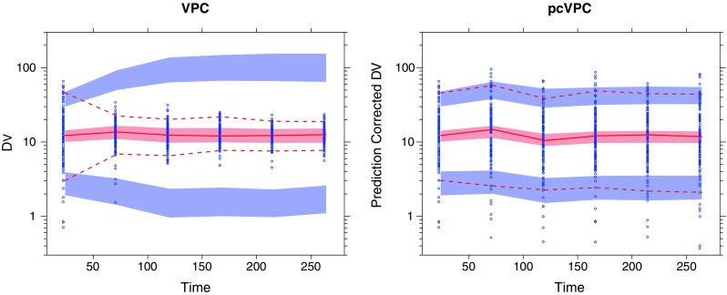
Example with a posteriori dose adaptation (TDM) based on observed trough plasma concentration (units per liter) monitoring over time. Traditional VPC (left) and pcVPC (right), with 95% interpercentile range, for the true model applied to a simulated dataset. Taken from: “Prediction-Corrected Visual Predictive Checks for Diagnosing Nonlinear Mixed-Effects Models”
However, until recently, I was not aware of how to perform these VPCs since the dependent variable changes and it all seemed way more complicated than a ‘simple’ scatter/percentile/confidence interval VPC. This post will therefore show how to create a pcVPC with a simulated dataset, in R, from scratch using a NONMEM model.
In addition to this post, PsN has some amazing functions to quickly generate your VPC. More information on how to create your VPC’s with PsN can be found on: https://uupharmacometrics.github.io/xpose/articles/vpc.html
Formula for prediction correction
As a very brief summary, as the name suggest, a prediction corrected VPC corrects each observation (or simulated observation) for the individual population prediction. Furthermore, it normalizes around the population prediction of a bin.
The following formula is used:
where, Yij is the observation, PREDbin is the median population prediction of the bin and PREDij is the population prediction of the observation. All resulting in the prediction corrected observation (pcYij).
The lbij in this formula is a baseline (which can be useful in PD modelling). However, this will not be used in this example.
Data simulation
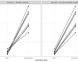
Our simulation was a two cohort simulation with 20 subjects per cohort (dosed 1 mg/kg or 3 mg/kg) with a strong linear covariate relationship on clearance (CL70kg = 7 L/h, slope= 0.15 L/h/kg). Samples were taken around a protocol time. The figure below shows the data for each individual:

There are two ways to perform the simulation needed to create the pcVPC. 1) Use the $SIMULATION block in NONMEM or 2) Use the vpc function in PsN.
For option 1, we fix our estimated parameters and change the $EST block to a $SIM block, and specify the number of simulations. Make sure that your output $TABLE contains at least the ID, MDV, TIME, DV and PRED.
The following $SIM block will simulate the original dataset 500x with the estimated model parameters and specified distribution:
$SIMULATION (20180921) ONLYSIM SUBPROBLEMS=500
Option 2 requires a slight modification compared to the command used in
previous posts. The reason is that the standard vpc command in PsN does not simulate the PRED column (which we need to create a PREDiction corrected VPC…). So in order to simulate the PRED column, we need to add the -predcorr argument as follows:
vpc -samples=500 -no_of_bins=8 -bin_by_count=1 -dir=vpc_Model1 Model1.mod -predcorr
In the rest of the post I will use this option in the R code presented below.
Many thanks to Mario Gonzales for advising me on the use of -predcorr!
R-script simulations
Much of the R code shown here is build upon previous tutorials on the generation of the other VPC’s. If something is unclear, I can advise you to go back to the other posts before diving in the pcVPC directly.
We first set some initial objects that we will use later on. We also specify the confidence interval and prediction intervals and the bin times. The bin times are needed to group observations together if not all the samples were taken at the same time points.
## Load libraries library(ggplot2) library(xpose) library(dplyr)######################################### # Set working directory of model file setwd("J:\\EstimationModel")
Number_of_simulations_performed <- 500 ## Used as 'samples' argument in PsN vpc function. Needs to be a round number.
######################################### # Set the prediction intervals
PI <- 80 #specify prediction interval in percentage. Common is 80% interval (10-90%) CI <- 95 #specify confidence interval in percentage. Common is 95
# Make a vector for upper and lower percentile perc_PI <- c(0+(1-PI/100)/2, 1-(1-PI/100)/2) perc_CI <- c(0+(1-CI/100)/2, 1-(1-CI/100)/2)
######################################### # Specify the bin times manually
bin_times <- c(0,3,5,7,10,14,18)
Number_of_bins <- length(bin_times)-1
We then search for the created simulation by PsN and read it using the xpose function read.nm.tables() and only select the observations (MDV ==0). We also need to create a new column which specifies from which of the 500 replicates the simulations originate and link the bin number with the observations.
#########################################
######### Load in simulated data

## Search for the generated file by PsN in the sub-folders
files <- list.files(pattern = "1.npctab.dta", recursive = TRUE, include.dirs = TRUE)

# This reads the VPC npctab.dta file and save it in dataframe_simulations
dataframe_simulations <- read_nm_tables(paste('.\\',files,sep=""))
dataframe_simulations <- dataframe_simulations[dataframe_simulations$MDV == 0,]


## Set the replicate number to the simulated dataset
dataframe_simulations$replicate <- rep(1:Number_of_simulations_performed,each=nrow(dataframe_simulations)/Number_of_simulations_performed)


# Set vector with unique replicates
Replicate_vector <- unique(dataframe_simulations$replicate)


#########################################
######### Create bins in simulated dataset


### Set bins by backward for-loop
for(i in Number_of_bins:1){
dataframe_simulations$BIN[dataframe_simulations$TIME <= bin_times[i+1]] <-i
}
An important value to calculate is the population prediction (PREDbin) per bin. This will be done using a piping function in which we select only the data from the first replicate to save some time. Hence, the population prediction will be equal for each replicate since we did not incorporate any parameter uncertainty in the simulation.
## Calculate median PRED per bin
PRED_BIN <- dataframe_simulations[dataframe_simulations$replicate ==1,] %>%
group_by(BIN) %>% # Calculate the PRED per bin
summarize(PREDBIN = median(PRED))
We can then merge this with our simulated dataset and calculate the prediction corrected simulated observations (PCDV).
dataframe_simulations <- merge(dataframe_simulations,PRED_BIN,by='BIN')
# Calculate prediction corrected simulated observations (PCDV)
dataframe_simulations$PCDV <- dataframe_simulations$DV *(dataframe_simulations$PREDBIN/dataframe_simulations$PRED)dataframe_simulations <- dataframe_simulations[order(dataframe_simulations$replicate,dataframe_simulations$ID,dataframe_simulations$TIME),]
We use this PCDV to calculate the prediction intervals and the confidence intervals as we have previously done which are the final calculations after which we have our simulated dataset ready.
sim_PI <- NULL
## Calculate predictions intervals per bin
for(i in Replicate_vector){
# Run this for each replicate
sim_vpc_ci <- dataframe_simulations %>%
filter(replicate %in% i) %>% # Select an individual replicate
group_by(BIN) %>% # Calculate everything per bin
summarize(C_median = median(PCDV), C_lower = quantile(PCDV, perc_PI[1]), C_upper = quantile(PCDV, perc_PI[2])) %>% # Calculate prediction intervals
mutate(replicate = i) # Include replicate number
sim_PI <- rbind(sim_PI, sim_vpc_ci)
}
###########################
# Calculate confidence intervals around these prediction intervals calculated with each replicate
sim_CI <- sim_PI %>%
group_by(BIN) %>%
summarize(C_median_CI_lwr = quantile(C_median, perc_CI[1]), C_median_CI_upr = quantile(C_median, perc_CI[2]), # Median
C_low_lwr = quantile(C_lower, perc_CI[1]), C_low_upr = quantile(C_lower, perc_CI[2]), # Lower percentages
C_up_lwr = quantile(C_upper, perc_CI[1]), C_up_upr = quantile(C_upper, perc_CI[2]) # High percentages
)
### Set bin boundaries in dataset
sim_CI$x1 <- NA
sim_CI$x2 <- NA
for(i in 1:Number_of_bins){
sim_CI$x1[sim_CI$BIN == i] <-bin_times[i]
sim_CI$x2[sim_CI$BIN == i] <-bin_times[i+1]
}
R-script observations
Our observations dataset can be loaded as a .csv file after which we select only the observations (CMT == 2 in this case).
In order to calculate the PCDV, we also need to apply the correction to our observations. For this, we need to have the PRED at each observation. We can do this by selecting the rows of the dataframe_simulations (row 1 until the number of observations in the original dataset).
############################################################
######### Read dataset with original observations
Obs <- read.csv("VPC.Estimation.Dataset.csv")Obs<- Obs[Obs$MDV == 0,]
### Add the population prediction to each observation (only use the data from 1 replicate)
Rep1 <- dataframe_simulations[
dataframe_simulations$replicate ==1,c("ID","TIME","PRED")]
Obs <- merge(Obs,Rep1,by=c("ID","TIME"))
We then add the bin numbers to the dataset, merge the population prediction per bin and calculate the PCDV.
#########################################
######### Create bins in original dataset### Set bins by backward for loop
for(i in Number_of_bins:1){
Obs$BIN[Obs$TIME <= bin_times[i+1]] <-i
}## ADD PRED BIN TO OBSERVATIONS
Obs <- merge(Obs,PRED_BIN,by='BIN')Obs$PCDV <- Obs$DV *(Obs$PREDBIN/Obs$PRED)
We can use the PCDV for the calculation of the percentiles which are going to compare with the simulated distributions.
############################################ ## Calculate confidence intervals of the observationsobs_vpc <- Obs %>% group_by(BIN) %>% ## Set the stratification identifiers (e.g. TIME, DOSE, CMT, BIN) summarize(C_median = median(PCDV, na.rm = T), C_lower = quantile(PCDV, perc_PI[1], na.rm = T), C_upper = quantile(PCDV, perc_PI[2], na.rm = T))
## Get median time of each bin of observations for plotting purposes bin_middle <- Obs %>% group_by(BIN) %>% summarize(bin_middle = median(TIME, na.rm = T))
# As a vector bin_middle <- bin_middle$bin_middle
obs_vpc$TIME <- bin_middle
We now have all the data we need to generate our pcVPC :).
Plotting
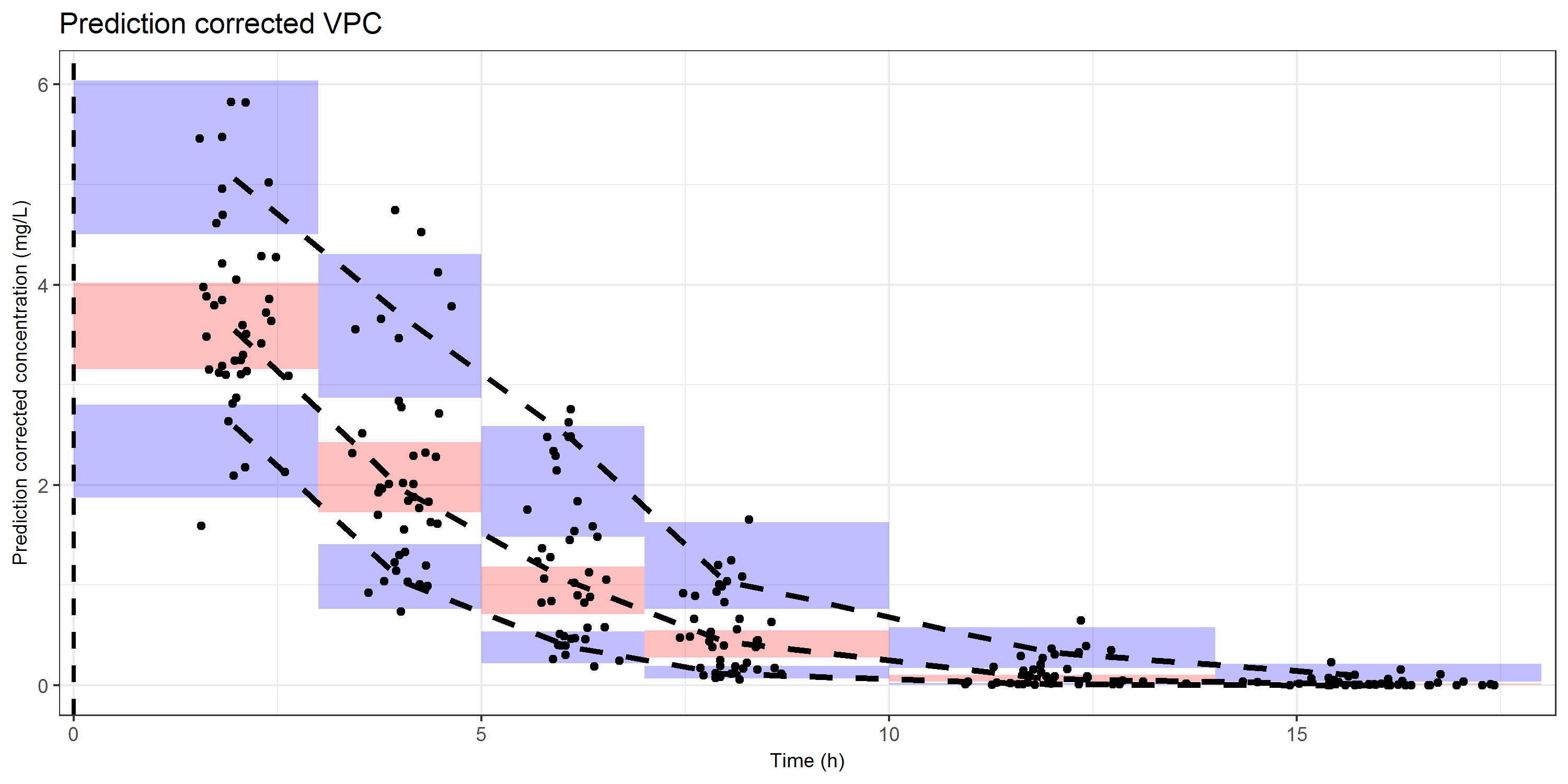
The ggplot object that will be generated is actually the same as for the confidence interval VPC. We have rectangles (shaded areas) for the distribution of the simulations, lines for the distribution of the data, and dots for the observed prediction corrected concentrations.
### VPC on a linear scale
CI_VPC_lin <- ggplot() +## Set bins
geom_rect(data=sim_CI, mapping=aes(xmin=x1, xmax=x2, ymin=C_median_CI_lwr, ymax=C_median_CI_upr), fill='red', alpha=0.25) +
geom_rect(data=sim_CI, mapping=aes(xmin=x1, xmax=x2, ymin=C_low_lwr, ymax=C_low_upr), fill='blue', alpha=0.25) +
geom_rect(data=sim_CI, mapping=aes(xmin=x1, xmax=x2, ymin=C_up_lwr, ymax=C_up_upr), fill='blue', alpha=0.25) +# Lines of the observations
geom_line(data = obs_vpc, aes(TIME, C_median), col = 'black', linetype = 'dashed', size = 1.25) +
geom_line(data = obs_vpc, aes(TIME, C_lower), col = 'black', linetype = 'dashed', size = 1.25) +
geom_line(data = obs_vpc, aes(TIME, C_upper), col = 'black', linetype = 'dashed', size = 1.25) +###### Add observations
geom_point(data = Obs,aes(x=TIME,y=PCDV),color='black')+####### Set ggplot2 theme and settings
theme_bw()+
theme(axis.title=element_text(size=9.0))+
theme(strip.background = element_blank(),
strip.text.x = element_blank(),legend.position="none") +# Set axis labels
labs(x="Time (h)",y="Prediction corrected concentration (mg/L)")+# Add vertical lines to indicate dosing
geom_vline(xintercept = 0, linetype="dashed", size=1) +# Set axis
#scale_y_log10(expand=c(0.01,0))+
scale_x_continuous(expand=c(0.01,0))+## Add title and subtitle
ggtitle("Prediction corrected VPC")#####################################
## Save as png
png("Figure_Simulation_Prediction corrected_VPC_with_Observations.png",width = 10, height = 5, units='in',res=300)print(CI_VPC_lin)
dev.off()
Tip
A prediction corrected VPC is commonly created on sparse sampled data. Instead of using the sampling time, one could also use the time after the most recent dose. This would give a clear picture about the distribution of your observations and how it compares to the distribution kinetics (majority in distribution phase, elimination phase, etc).
Note on the used terminology:
A recent NMusers thread contained a discussion on the terminology that we use to describe our VPC compared to the actual statistical meaning, which may differ. Please find an informative reply from Mike Smith on this topic below:
“As Mats and Bill point out [former replies], the common usage within our community is to say that the percentiles (5th, 95th) are “prediction intervals” and the interval estimates / uncertainty around these percentiles are “confidence intervals”. But as Ken points out [former reply], these terms do not strictly correspond to the statistical definition of each if you take into account what the VPC procedure is actually doing. The VPC is a model diagnostic procedure for the observed data and provides a visual check of whether the model is capturing central tendencies and dispersion in our data. (BTW, I *know* there are debates about the usefulness or otherwise of VPC plots. I’m not going to address that here and I suggest we don’t disappear down *that* rabbit hole.)
We are NOT trying to make probabilistic statements about the likelihood of observed percentiles being within the intervals around these. So if the question arises from some reviewer based on our use of statistically woolly terms like “prediction interval” or “confidence interval” we should be ready to put up our hands and admit that the terms we are using do not imply those statistical properties. We could advocate changing the terminology used, but that may not have traction in the community after this length of time. But we *should* be cognizant about what these things are, what they’re for, what the formal, statistical terminology implies and what our use (or maybe misuse) is or isn’t implying.”
COMMENT
Any suggestions or typo’s? Leave a comment or contact me at info@pmxsolutions.com!


Hi Michiel,
Excellent page and work!
You can add the PRED column to the output in PsN with the following argument: -predcorr. Please see: https://uupharmacometrics.github.io/xpose/articles/vpc.html for reference (section Creating the VPC using a PsN folder).
Best regards,
Mario
Dear Mario,
Thank you for your comment. This much faster option has now been added to the post!
Michiel
Hi Michiel,
I’m so glad to find your blog. Can you please help me understand the necessity of adding variability correction (pvcVPC in the same paper)? I read the paragraph about pvcVPC multiple times over the years but still cannot understand it.
If you don’t already know, pvcVPC can be done using PsN argument: -varcorr.
Best regards,
DY
Dear DY,
Great question, I must admit that I have read the paper multiple times but did not spend any attention on the pvcVPC. I can only imagine it plays a role when you have additive residual errors, in which a larger residual component play a role in the lower concentrations compared to the higher concentrations in a bin, which we should correct for.
However, I have never seen a paper publish this pvcVPC so I don’t know if it is actually being implemented nor have I created them myself.
Sorry that I can’t be of any further assistance.
Michiel
Hi
How to generate VPC with time after dose
Regards
Alex
Hello Alex,
The easiest way is to make sure that your original dataset has a TAD column. This can then be used to merge/replace the TIME column in the code. Also the bins should then be calculated on the TAD values and not on the TIME column.
Michiel