Introduction
We are not all the same. We know that there is variability originating from physiological differences in the pharmacokinetic and pharmacodynamic (PK/PD) processes between individuals in a population, also called the inter-individual variability or IIV. We also know that the there can be changes in these processes from one day to another, or between two dose administrations, which is called the inter-occasion variability or IOV. Fortunately, both can be quantified and can be included in our models! If we have the right data.
IIV and IOV
If we quantify differences in the volume of distribution of a drug in multiple individuals, we call this IIV. This means that each individual has a slightly different volume, centered around a typical value, but this volume remains equal within the same individual, even when the drug is administered on multiple occasions.
However, it is also possible that when we for example give a drug orally, the absorption rate constant or bio-availability is slightly different in the same individual dependent on if the individual just had breakfast, is fasted, had a glass of cold water, etc. This means that between each dose administration there is variability within the same subject, called IOV.
Single dose data
What happens when we only have data after a single dose? Can we quantify both IIV and IOV? If there is no literature data to further assist us, the answer is no. Let’s have a look at why this is not possible.
When we get the data, we build a population PK model and observe that the absorption rates significantly differ between individuals. Hence, we see different absorption profiles for each individual. This means that we can (try to) estimate the variance in the model on this parameter as IIV and judge whether this gives a significant improvement in the model fit.
In the figure below you can see what this inclusion of IIV might look like. The colored circles represent individuals 1-5. Furthermore, we have a certain typical absorption rate constant of 1.5/h and each individual has its own rate constant on a normally distributed curve (not drawn as log-normal for convenience).

Impact on simulations
The scenario discussed above is quite common. We build a model on available data, we estimate the IIV, we report the parameters, and write the manuscript. The underlying assumption of subsequent simulations with this model is that the variability exists between individuals only. Hence, an individual will have exactly the same absorption rate on the next day.
In order to visualize this, I simulate multiple dose administrations with only IIV on the absorption rate constant parameter for 6 random individuals. As you can see, subject number 15 has a lower Cmax and a slightly longer Tmax than the others, indicating that this individual has the lowest absorption rate constant. Since it is included in the model as IIV, this subject is consistently lower after each dose administration over the full 48h dosing period. However, part of this variability might be explained as IOV.

Multiple dose data
In the previous example, we only had data from a single occasion, limiting the information we can obtain to solely the IIV. If you want to quantify whether you can stratify the total level of variability in both IIV and IOV, you at least need to have data on two occasions, preferably more, within the same individual.
Let’s get back the individuals from the single ascending dose study and give them the same drug another time, quantify the IIV, quantify the BOV, and plot the individual absorption rates per occasion again.

What we observe in the figure above is that the second circle of each individual is not close to the first circle, it is actually quite far apart. This indicates that the absorption rate constants of both occasion are completely different and there is quite some variability present. However, if we look at the bars, representing the ‘average’ individual absorption rate constants, these are quite close to the median.
This means that when we added data from the second occasion and quantified the different levels of variability, the IIV is low but the level of IOV is high!
Impact on simulations

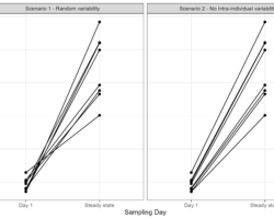
Sowhat happens in the scenario when we simulate with no IIV but only with the quantified IOV? Suddenly the profiles of each individual look completely different than what we had before! Compared to 1 individual being consistently under- or over-exposed, the absorption rates now changes between doses and an individual may have the lowest Cmax on one occasion but the highest on another. As you can imagine, dependent on what kind of efficacy matrix you are simulating in your clinical trial simulation, this may significantly impact your results.
If we are simulating a drug that requires a certain average concentration over time, or a time above a certain threshold, both simulations will give completely different results which should be taken into account. This is one of the risks of simulating multiple dosing regimens when the model has been developed solely on single dose data.
However, since both measures contain variability on the same parameter, the total variability in the population will remain the same and will therefore not influence your prediction interval.
Of course, the other way around can also occur. In which the majority of the variability originates from inter-individual differences and the absorption rate constant within an individual is similar. If this is the case, simulations would look similar to before (with high IIV an low/no IOV).

Parameter identification
But is it always possible to quantify the IIV and IOV with low RSE’s if we have data from multiple occasions in the same individual? Hopefully you can imagine that it is a little bit more complicated. If there is a high level of IIV and a low level of IOV, or vice versa, it may be impossible to quantify one of the components. Furthermore, if only sparse samples are being taken in the absorption phase, it may become even more difficult to correctly quantify this parameter and the level of variability around it. Addition of IIV and IOV on this parameter may therefore result in high RSE’s and a high condition number, indicating possible overparameterization of your model.
mrgsolve with IOV
Multiple methods exist to simulate IOV in mrgsolve. Compared to writing each occasion separately, as I normally do in NONMEM, I really prefer this method:
https://github.com/metrumresearchgroup/mrgsolve/issues/408
COMMENT
Any suggestions or typo’s? Leave a comment or contact me at info@pmxsolutions.com!
Continue reading:
- From Animals to Algorithms: Leveraging PK/PD Models to Drive the 3R’s in Pharmacology

- Exploration of intra-individual variability in a multiple dose study during NCA
- A pharmacometrician’s job interview: the case study