A non-compartmental analysis (NCA) is commonly performed to analyse the data of a pharmacokinetic study. It is an easy way of getting your pharmacokinetic parameters (such as the Cmax, tmax, AUC, etc.) without having to perform any advanced modelling techniques. If sufficiently dense data is collected, we can determine the PK parameters on an individual level and summarise them as means, standard deviations, geometric means and/or ranges, whatever was specified in our analysis plan. These summary statistics show how the average in the population behaves but also the inter-individual variability across your population, an important component for future decisions, especially if a narrow therapeutic window exists. However, is that always the inter-individual variability we are looking at?
Intra- or inter-individual variability?
A NCA usually provides sufficient quantitative information to be reported, but sometimes in multiple dose studies (when you have two or more profiles in the same individual) we see a high degree of variability in our population on both days and we wonder, are individuals that have an above average PK on day 1 also above average at steady state (indicating low intra-individual variability), or are they randomly scattered across the days (indicating high day-to-day variability)?
Having this information allows us to better understand the source of the variability. For example, if individuals keep the same rank order across days, it might be related to the rate of individual clearances that are genetically defined causing a significant inter-individual variability but low intra-day variability for the same individual, hence, dosing might need to be altered for some individuals. If individual exposures changes between days and the rank order changes, this may indicate a random source of variability that is independent on the subject characteristics, in this case, dosing adjustments based on the day 1 PK profile should not be made as the PK profile on later days can be below the mean at identical doses. Perhaps the absorption of the drug changes from day to day or the dissolution is highly variable?
This analysis can be performed by advanced statistical methods and population PK modelling, but as a NCA is most often a crude analysis of the data at an early stage immediately after study execution this blog post provides some of the figures and simple calculations one can do to identify whether the variability is driven by inter- or intra- individual variability.
Explanation:
- Intra = within-subject
- Inter = between-subject
Objective
In this post we will explore two cases, a case with normal day-to-day variability (no clear correlations between exposures on Day 1 and later) and one with no intra-individual variability (individuals with high exposures on Day 1 will keep high exposures). It will also present the difficulties of seeing these differences when only looking at the summary results of a NCA. As always, this post will also include the R code used to generate the figures.
Datasets and exploration
The following example datasets provide the Cmax values of 8 individuals on Day 1 and at steady-state in both scenarios, scenario 1 – Random intra-individual variability and scenario 2 – No Intra-individual variability.
Dataset scenario 1 – Random variability
| Subject ID | Cmax (ng/mL) | |
| Day 1 | Steady-state | |
| 1 | 7.97 | 49.86 |
| 2 | 10.63 | 39.30 |
| 3 | 8.18 | 37.65 |
| 4 | 7.18 | 51.99 |
| 5 | 12.93 | 30.18 |
| 6 | 9.55 | 52.11 |
| 7 | 10.14 | 36.57 |
| 8 | 7.15 | 58.32 |
| Mean (ng/mL) | 9.2 | 44.5 |
| Standard deviation (ng/mL) | 2.0 | 9.8 |
| Coefficient of variation (%) | 22 | 22 |
Dataset scenario 2 – No Intra-individual variability
| Subject ID | Cmax (ng/mL) | |
| Day 1 | Steady-state | |
| 1 | 7.97 | 37.65 |
| 2 | 10.63 | 52.11 |
| 3 | 8.18 | 39.30 |
| 4 | 7.18 | 36.57 |
| 5 | 12.93 | 58.32 |
| 6 | 9.55 | 49.86 |
| 7 | 10.14 | 51.99 |
| 8 | 7.15 | 30.18 |
| Mean (ng/mL) | 9.2 | 44.5 |
| Standard deviation (ng/mL) | 2.0 | 9.8 |
| Coefficient of variation (%) | 22 | 22 |
Important conclusion: If you look at these tables, one would not notice any differences upon first inspection. The mean, standard deviation, and coefficients are the same across both scenarios. There is some accumulation (9.2 ng/mL to 44.5 ng/mL) from Day 1 to steady-state but this is again identical in both scenarios.
However, as soon as we start exploring the data in R and create some scatter plots with the Cmax per day and individual lines, we start seeing some interesting things.
# dfCmax contains the Subject ID and the Cmax per day in the long format

ggplot(dfCmax,aes(x=Day,y=value,group=Subject.ID))+
  geom_point()+
  geom_line()+
  facet_wrap(~Scenario)+
  theme_bw()+
  ylab('Cmax (ng/mL)')+
  xlab('Sampling Day')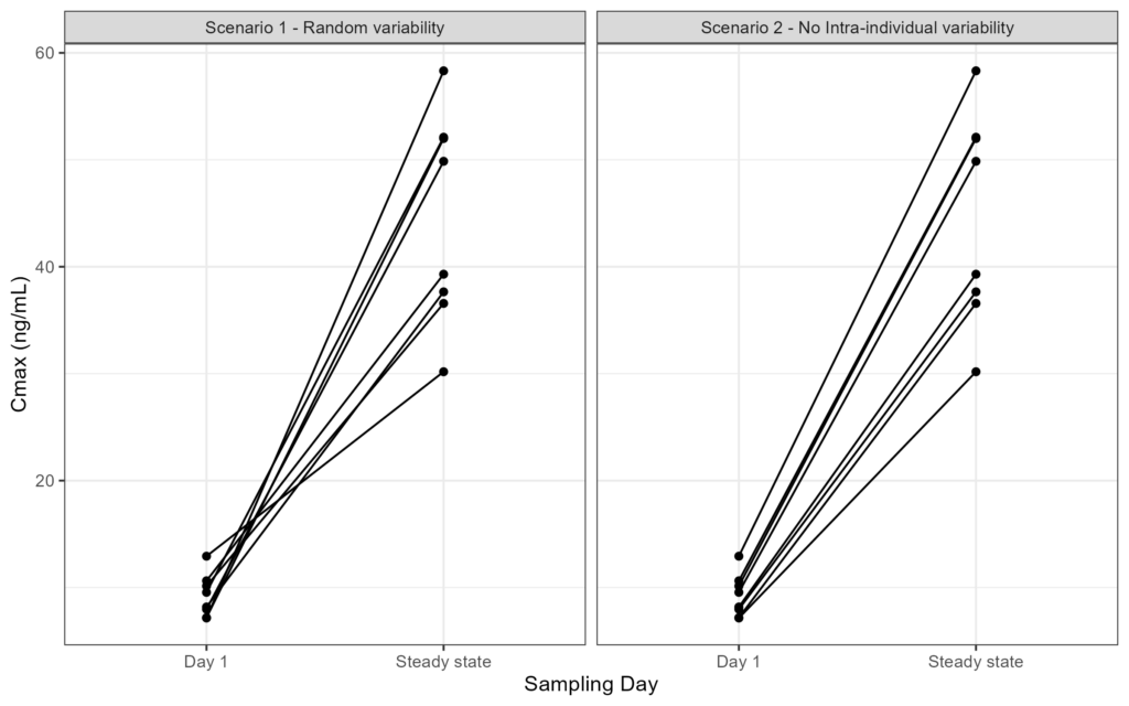
As you can see in the figure on the left, multiple lines cross. This indicates that an individual that has a high concentration on day 1 is lower at steady state, or vice versa. However, the figure on the right presents an extreme scenario in which all individuals kept the same order of exposures as they started on Day 1. I do mention that this is an extreme scenario as one will most likely have some kind of variability present in the dataset.
Both scenarios that are presented here gave similar results when looking at the summary statistics, but the origin of the variability can only be understood when looking at the results on an individual level.
Determining the rank order
We can even better understand and quantify what is happening when we start ranking the individual Cmax values on Day 1 and at steady-state. To calculate the maximum number of total changes that can happen in theory with 8 individuals, we need to think about all the possible changes in their rankings. Given 8 individuals, the biggest possible shift occurs when someone moves from the highest to the lowest position or vice versa. Each individual can potentially move from one rank to any other rank, and the total change will be the absolute sum of all these shifts.
The maximal number is obtained by a full reversal, a full reversal means that every individual swaps places with their exact opposite in the ranking. For example:
- The person originally in 1st place moves to 8th place.
- The person in 2nd place moves to 7th place.
- The person in 3rd place moves to 6th place, and so on.
Calculating the Total Changes
To find the total change, we need to calculate how many places each individual has moved.
Let’s calculate the maximal movement for each subject:
- The person who was in 1st place moves to 8th place: change = 7
- The person who was in 2nd place moves to 7th place: change = 5
- The person who was in 3rd place moves to 6th place: change = 3
- The person who was in 4th place moves to 5th place: change = 1
Similarly, for the other half:
- The person who was in 8th place moves to 1st place: change = 7
- The person who was in 7th place moves to 2nd place: change = 5
- The person who was in 6th place moves to 3rd place: change = 3
- The person who was in 5th place moves to 4th place: change = 1
The total maximal change for all 8 individuals is: 7+5+3+1+7+5+3+1=32
This configuration results in the largest possible change because every individual has swapped places with the person furthest from them in rank, maximizing the absolute distance moved. Any other arrangement of changes would result in a smaller total movement. Hence, this is the scenario where the total change reaches its theoretical maximum. If this theoretical maximum is reached, there is a very high level of intra-individual variability.
We can now look at how that applies to our dataset where the ranking has been added for Scenario 1:
| Subject ID | Cmax (ng/mL) | Rank | |||
| Day 1 | Steady-state | Day 1 | Steady-state | Delta | |
| 1 | 7.97 | 49.86 | 6 | 4 | 2 |
| 2 | 10.63 | 39.3 | 2 | 5 | -3 |
| 3 | 8.18 | 37.65 | 5 | 6 | -1 |
| 4 | 7.18 | 51.99 | 7 | 3 | 4 |
| 5 | 12.93 | 30.18 | 1 | 8 | -7 |
| 6 | 9.55 | 52.11 | 4 | 2 | 2 |
| 7 | 10.14 | 36.57 | 3 | 7 | -4 |
| 8 | 7.15 | 58.32 | 8 | 1 | 7 |
| Absolute delta | 30 | ||||
| Maximal theoretical difference | 32 | ||||
| Rank Change Coefficient | 0.94 | ||||
As we sum the absolute delta’s from our dataset, we see an absolute delta of 30, close to the maximal theoretical difference of 32. We can observe that there is quite a high Rank Change Coefficient of 0.94 (maximal is 1, calculated by the absolute delta divided by the maximal theoretical difference), indicating a very low correlation between the individual exposures on Day 1 and steady state. If we would have looked at Scenario 2, where the rank order remained the same across days, the delta would be 0 and the Rank Change Coefficient would also be 0, as none of the individual switched places.
In case of a high rank change coefficient, there is a high level of intra-individual variability. In the case of a low rank change coefficient, there is still significant inter-individual variability, with minimal to no intra-individual variability.
Note: The Rank Change Coefficient is not a statistical parameter, there are many ways to calculate the differences between ranks but I find this the most easy to interpret the comparison across days
Summary
A NCA provides valuable information on the characteristics of a PK curve and is a crucial tool in pharmacokinetic analyses. However, looking only at the summary statistics might obscure if we are dealing with high or low intra-individual variability across days. This information is key in driving future decision making or future model development but is commonly overlooked in the reporting.
If your coefficient of variation is high enough that you need to check what are potential sources of the variability, this information can be easily obtained by:
- Visualizing the correlation between both days with individual trend lines in a scatter plot
- Calculating the Rank Change Coefficient across days
I would propose to have a section on this in every NCA report in which multiple dose data is collected in the same individuals.
What more would you look at to investigate this?
Any suggestions or typo’s? Leave a comment or contact me at info@pmxsolutions.com!